
An important goal of statistics and machine learning is to find patterns in data and explore potential relationships between variables (or features). A well-known approach to achieve that is to use regression models, including polynomial regressions.
The objective of this blog post is to highlight the limitation of polynomial regressions for some datasets.
For illustration, we consider the dataset displayed in Figure 1.
These data depict the value of the acceleration over time in an experiment about the efficacy of helmets in a motor-cycle crash. Full details about the dataset can be found in Silverman (1985), and the dataset itself is available in the MASS package in R.
We want to summarise the variability of acceleration (\(y\) ) as a function of time (\(x\)).
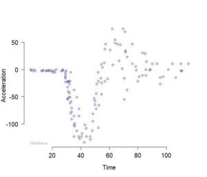
Figure 1: Values of the acceleration (in \(9.81m/s^2\)) taken through time (in milliseconds) in an experiment on the efficacy of helmets for a motor-cycle crash.
Let us denote by \(y_i\) the observed values of the acceleration at time points \(x_i, \;i=1,…,n\).
The simplest regression model for these data assumes that the data come from a simple linear process as follows
\[ y_i = f(x_i) + \varepsilon_i, \quad i=1,…,n, \]
where \(f\) is the linear preditor function given by
\[f(x)=\alpha_0 + \alpha_1 x,\;\;\; \alpha_0,\alpha_1\in \mathbb{R},\]
and \(\varepsilon_i\) is the noise or error term.
The intercept and slope coefficients \(\alpha_0\) and \(\alpha_1\) can be estimated via the method of least squares by minimising the RSS function given by
\[RSS(\alpha_0,\alpha_1)=\sum_{i=1}^n(y_i-\alpha_0-\alpha_1x_i)^2\]
For the motor-cycle data shown in Figure 1, we find \(\alpha_0=-53.0\) and \(\alpha_1=54.5\).
The corresponding fitted line is shown in Figure 2.
Clearly, this line does not suit the data.
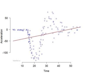
Figure 2: Straight line fitted to the motor-cycle data.
One way to obtain a better fit is to drop the simple straight line and use some \(p\)-degree polynomial instead. That is:
\[
f(x)=\sum_{r=0}^p\,\alpha_r \, x^r,
\]
where the unknown coefficients \(\alpha_r\) can be estimated by the method of least squares.
The fitted polynomial curves corresponding to different values of \(p\) are shown in Figure 3.
Although these fitted curves are closer to the data points overall compared to the straight line in Figure 1, Figure 3 does give a glimpse of the limitation of the polynomial approach regarding complex data patterns.
In particular, increasing the degree of the polynomial tend to cause some instability of the fitted curve, especially towards the edges. This behaviour/drawback of polynomial curves is caused by the global dependence of the polynomial terms on local properties of the data.
In other words, an individual observation can exert an unexpected influence on remote parts of the polynomial terms, and such behaviour can lead to an unstable curve with poor interpolation and extrapolation properties, as illustrated in Figure 3.
An attractive way of circumventing this problem is to use appropriate smoothing methods.
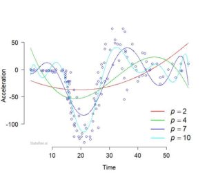
Figure 3: Polynomial curves of degree \(p\) fitted to the motor-cycle data.
In the up coming blog pots, we shall explore several smoothing methods and illustrate how some of them allow to tackle the pitfalls of polynomial regressions.
References
- Venables W. N. and Ripley B. D. (2002). Modern Applied Statistics with S, Fourth Edition. Springer.
- Silverman B. W. (1985). Some aspects of the spline smoothing approach to non-parametric curve fitting. Journal of the Royal Statistical Society (Series B), 47:1–52.
- De Boor C. (1978). A practical guide to splines. Springer.